Randomized Outlier-Robust Fitting: The Random Sample Consensus (RANSAC) Learning Algorithm Applied to Image Stitching from Scratch
Article in progress
| Left Image | Right Image |
|---|---|
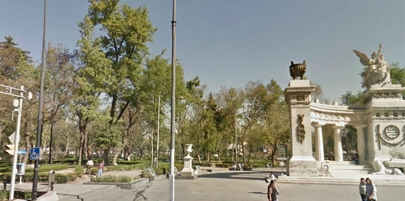 |
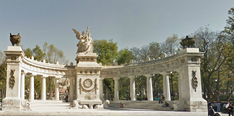 |
Consider two images of the same scene from difference perspectives. An object, like a statue or a person, in the underlying scene when viewed from different perspectives are related by a geometric transformation. A homography mapping is that transformation, affine and rotational. The image below shows the scene structure
| Homography Mapping |
|---|
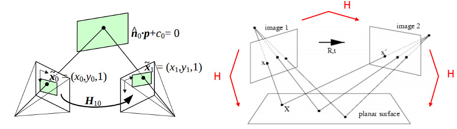 |
| Source: https://docs.opencv.org/master/d9/dab/tutorial_homography.html |
A mapping between two planes can be modeled as
\[\begin{bmatrix} x' \\ y' \\ 1' \\ \end{bmatrix} \sim \begin{bmatrix} h_{11} & h_{12} & h_{13}\\ h_{21} & h_{22} & h_{23}\\ h_{31} & h_{32} & h_{33} \end{bmatrix} \begin{bmatrix} x \\ y \\ 1 \\ \end{bmatrix}\]Where solutions,
\[x' = \frac{h_{11}x + h_{12}y + h_{13}}{h_{31}x + h_{32}y + h_{33}}\\ y' = \frac{h_{21}x + h_{22}y + h_{23}}{h_{31}x + h_{32}y + h_{33}}\]rearranged,
\[h_{11}x + h_{12}y + h_{13} - h_{31}xx' + h_{32}yx' + h_{33}x' = 0\\ h_{21}x + h_{22}y + h_{23} - h_{31}xy' + h_{32}yy' + h_{33}y' = 0\]Using 4 points for the estimation, the matrix becomes,
\[\begin{bmatrix} -x_1 & -y_1 & -1 & 0 & 0 & 0 & x_1 x_1' & y_1 x_1' & x_1'\\ 0 & 0 & 0 & -x_1 & -y_1 & -1 & x_1 y_1' & y_1 y_1'& y_1'\\ -x_2 & -y_2 & -1 & 0 & 0 & 0 & x_2 x_2' & y_2 x_2' & x_2'\\ 0 & 0 & 0 & -x_2 & -y_2 & -1 & x_2 y_2' & y_2 y_2'& y_2'\\ -x_3 & -y_3 & -1 & 0 & 0 & 0 & x_3 x_3' & y_3 x_3' & x_3'\\ 0 & 0 & 0 & -x_3 & -y_3 & -1 & x_3 y_3' & y_3 y_3'& y_3'\\ -x_4 & -y_4 & -1 & 0 & 0 & 0 & x_4 x_4' & y_4 x_4' & x_4'\\ 0 & 0 & 0 & -x_4 & -y_4 & -1 & x_4 y_4' & y_4 y_4'& y_4'\\ \end{bmatrix} \textbf{H} = \textbf{0}\]We can solve this system of equations, \(\mid\mid AH\mid\mid^2\) with \(\mid\mid H\mid\mid=1\). An SVD decomposition solves equations of type \(AX=0\) returning a set of orthonormal basis vectors conveniently enforcing \(\mid\mid X\mid\mid=1\).
##homography mapping givien a set of keypoints
def homography_mapping(kp1,kp2):
    #minimize ||AH||^2
    A = []
    for idx, pts in enumerate(kp1):
        x, y = np.array(pts,dtype=float)
        u, v = np.array(kp2[idx],dtype=float)
        A.append([x, y, 1, 0, 0, 0, -u*x, -u*y, -u])
        A.append([0, 0, 0, x, y, 1, -v*x, -v*y, -v])
    _, _, V = np.linalg.svd(np.array(A))
    V =  V[-1].reshape((3,3))
    V = V/V[2,2]
    return V
import numpy as np
import matplotlib
import matplotlib.pyplot as plt
from mpl_toolkits.mplot3d import Axes3D
from PIL import Image
from scipy.ndimage import gaussian_filter
from scipy.spatial.distance import cdist
from skimage.transform import ProjectiveTransform
from skimage.transform import warp
from skimage.transform import SimilarityTransform
from cv2 import warpPerspective
import cv2
###RANSAC loop for homography mapping
best_h = []
best_inliers = []
best_score = 0
best_residual = 0
for i in np.arange(8000):
    #a. select 4 random samples
    SAMPLE_PTS = 4
    pts = np.random.choice(np.arange(len(closest_pts_idx[0])),SAMPLE_PTS,replace=False)
    ###b. fit 4 feature pairs
    fet_im1 = np.array(kp1)[closest_pts_idx[0][pts]]
    fet_im2 = np.array(kp2)[closest_pts_idx[1][pts]]
    ##c. Homography mapping of a single point
    H_mat = homography_mapping(fet_im1,fet_im2)
    #d. get the inliers and the points with a distance less than 3
    # from the matched transform
    inliers = [] #inliers index
    res = 0
    for index in np.arange(len(closest_pts_idx[0])):
        a1 = np.array(kp1)[closest_pts_idx[0][index]]
        a2 = np.array(kp2)[closest_pts_idx[1][index]]
        vec1 = np.array([a1[0],a1[1],1])
        trans = np.dot(H_mat,vec1)
        trans = trans/trans[2]
        trans = [trans[0],trans[1], 1]
        error = np.sqrt(np.sum(((trans[0:2]-a2)**2)))
        if error < 15:
            inliers.append(index)
            res += error
    if best_score < len(inliers):
        best_score = len(inliers)
        best_h = H_mat
        best_inliers = inliers
        best_residual = res / best_score

print(f"best score: {best_score}, best Hmatrix: {best_h}, best residual: {best_residual}")
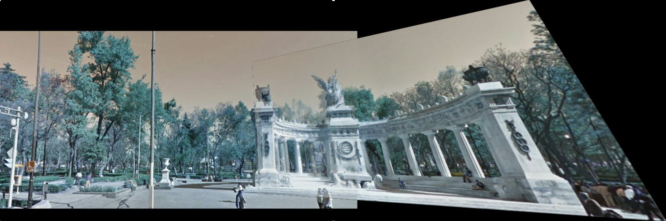
#merge overlaid images
def warp_images(image0, image1, transform):
    r, c = image1.shape[:2]
    # Note that transformations take coordinates in (x, y) format,
    # not (row, column), in order to be consistent with most literature
    corners = np.array([[0, 0],
                        [0, r],
                        [c, 0],
                        [c, r]])
    # Warp the image corners to their new positions
    warped_corners = transform(corners)
    # Find the extents of both the reference image and the warped
    # target image
    all_corners = np.vstack((warped_corners, corners))

    corner_min = np.min(all_corners, axis=0)
    corner_max = np.max(all_corners, axis=0)

    output_shape = (corner_max - corner_min)
    output_shape = np.ceil(output_shape[::-1])

    offset = SimilarityTransform(translation=-corner_min)

    image0_ = warp(image0, offset.inverse, output_shape=output_shape, cval=-1)

    image1_ = warp(image1, (transform + offset).inverse, output_shape=output_shape, cval=-1)

    image0_zeros = warp(image0, offset.inverse, output_shape=output_shape, cval=0)

    image1_zeros = warp(image1, (transform + offset).inverse, output_shape=output_shape, cval=0)

    overlap = (image0_ != -1.0 ).astype(int) + (image1_ != -1.0).astype(int)
    overlap += (overlap < 1).astype(int)
    merged = (image0_zeros+image1_zeros)/overlap
    im = Image.fromarray((255*merged).astype('uint8'), mode='RGB')
    im.save('stitched_images.jpg')
    im.show()
#plot figures
m1 = np.array(kp1)[closest_pts_idx[0][best_inliers]]
m2 = np.array(kp2)[closest_pts_idx[1][best_inliers]]

H_mat_all_inliers = homography_mapping(m1,m2)